Real data

When real data serves as input to a DFT, the resulting complex output data follows a special property, which is that about half of the output is redundant because it consists of complex conjugates of the other half. This is called Hermitian redundancy. So it’s only necessary to store the non-redundant part of the data. Most FFT libraries use this property to offer specific storage layouts for FFTs involving real data. rocFFT provides three enumeration values for rocfft_array_type to deal with real data FFTs:

• REAL: rocfft_array_type_real

• HERMITIAN_INTERLEAVED: rocfft_array_type_hermitian_interleaved

• HERMITIAN_PLANAR: rocfft_array_type_hermitian_planar

The REAL (rocfft_array_type_real) enumeration specifies that the data is purely real. This can be used to feed real input or get back real output. The HERMITIAN_INTERLEAVED (rocfft_array_type_hermitian_interleaved) and HERMITIAN_PLANAR (rocfft_array_type_hermitian_planar) enumerations are similar to the corresponding full complex enumerations in the way they store real and imaginary components but store only about half of the complex output. Client applications can perform a forward transform and analyze the output or they can process the output and do a backward transform to get real data back. This is illustrated in the following figure.

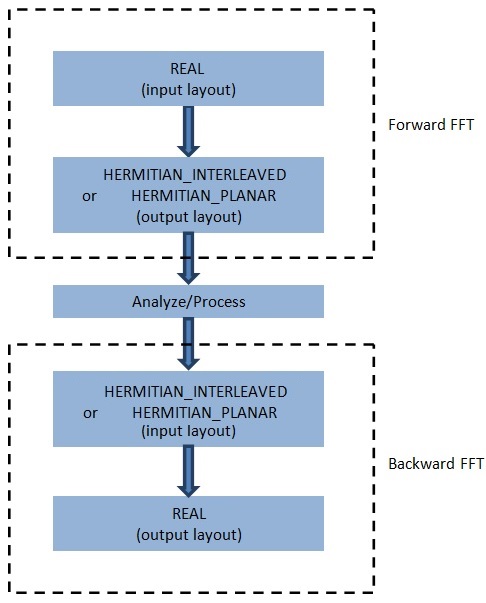
Fig. 1 Forward and backward real FFTs

Note

Real backward FFTs require that the input data be Hermitian-symmetric, which would naturally happen in the output of a real forward FFT. rocFFT will produce undefined results if this requirement is not met.

Consider the full output of a 1D real FFT of length \(N\), as shown in following figure:

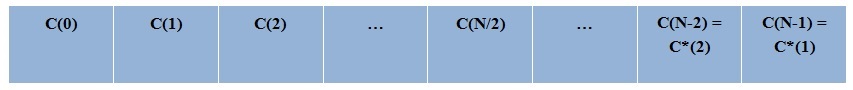
Fig. 2 1D real FFT of length N

Here, C* denotes the complex conjugate. Because the values at indices greater than \(N/2\) can be deduced from the first half of the array, rocFFT only stores the data up to the index \(N/2\). This means that the output contains only \(1 + N/2\) complex elements, where the division \(N/2\) is rounded down. Examples for even and odd lengths are given below.

An example for \(N = 8\) is shown in following figure.

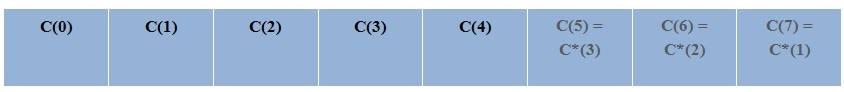
Fig. 3 Example for N = 8

An example for \(N = 7\) is shown in following figure.

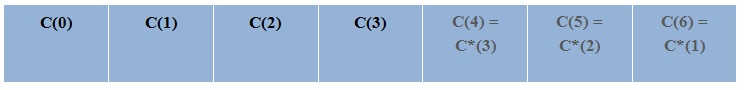
Fig. 4 Example for N = 7

For a length of 8, only \((1 + 8/2) = 5\) of the output complex numbers are stored, with the index ranging from 0 through 4. Similarly, for a length of 7, only \((1 + 7/2) = 4\) of the output complex numbers are stored, with the index ranging from 0 through 3. For 2D and 3D FFTs, the FFT length along the innermost dimension is used to compute the \((1 + N/2)\) value. This is because the FFT along the innermost dimension is computed first and is logically a real-to-Hermitian transform. The FFTs that are along other dimensions are computed next and are complex-to-complex transforms. For example, assuming \(Lengths[2]\) is used to set up a 2D real FFT, let \(N1 = Lengths[1]\) and \(N0 = Lengths[0]\). The output FFT has \(N1*(1 + N0/2)\) complex elements. Similarly, for a 3D FFT with \(Lengths[3]\), \(N2 = Lengths[2]\), \(N1 = Lengths[1]\), and \(N0 = Lengths[0]\), the output has \(N2*N1*(1 + N0/2)\) complex elements.

Supported array type combinations

Not in-place transforms:

• Forward: REAL to HERMITIAN_INTERLEAVED

• Forward: REAL to HERMITIAN_PLANAR

• Backward: HERMITIAN_INTERLEAVED to REAL

• Backward: HERMITIAN_PLANAR to REAL

In-place transforms:

• Forward: REAL to HERMITIAN_INTERLEAVED

• Backward: HERMITIAN_INTERLEAVED to REAL

Setting strides

The library requires the user to explicitly set input and output strides for real transforms for non-simple cases. See the following examples to understand which values to use for input and output strides under different scenarios. These examples show typical use cases, but you can allocate the buffers and choose a data layout according to your needs.

The following figures and examples explain the real FFT features of this library in detail.

This schematic illustrates the forward 1D FFT (real to Hermitian).

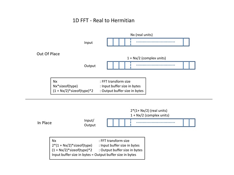
Fig. 5 1D FFT - Real to Hermitian

This schematic shows an example of a not in-place transform with an even \(N\) and how strides and distances are set.

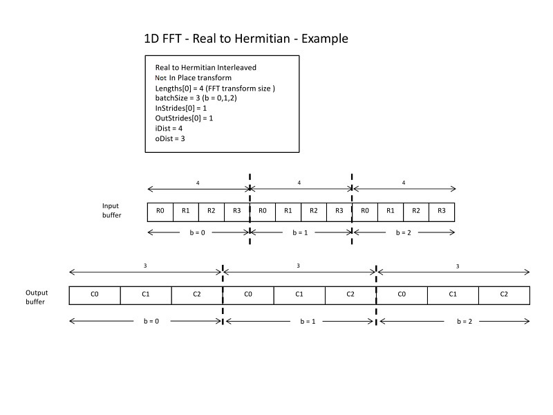
Fig. 6 1D FFT - Real to Hermitian: example 1

This schematic shows an example of an in-place transform with an even \(N\) and how strides and distances are set. Even though this example only deals with one buffer (in-place), the output strides/distance can take different values compared to the input strides/distance.

Fig. 7 1D FFT - Real to Hermitian: example 2

Here is an example of an in-place transform with an odd \(N\) and how strides and distances are set. Even though this example only deals with one buffer (in-place), the output strides/distance can take different values than the input strides/distance.

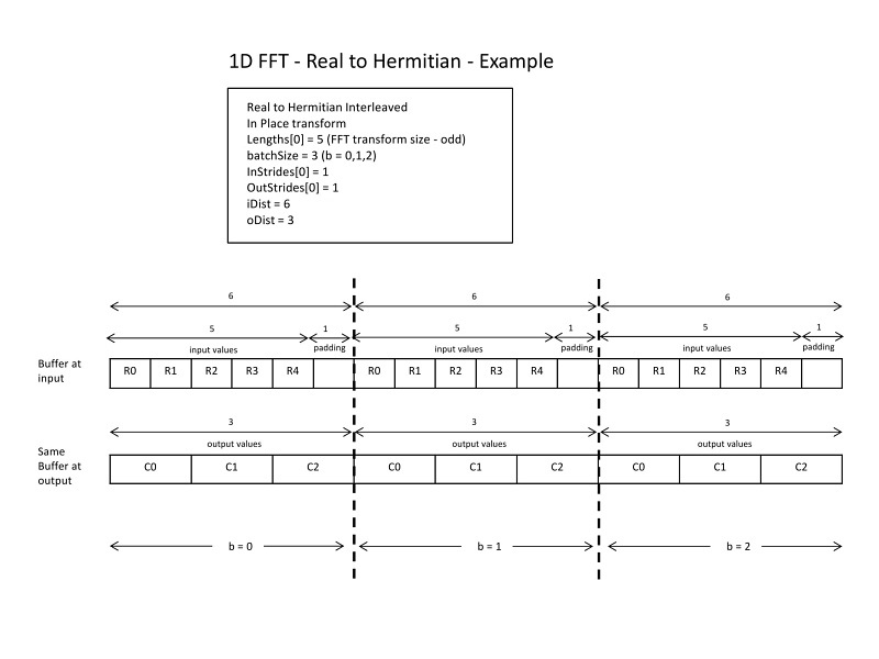
Fig. 8 1D FFT - Real to Hermitian: example 3

This schematic illustrates the backward 1D FFT (Hermitian to real).

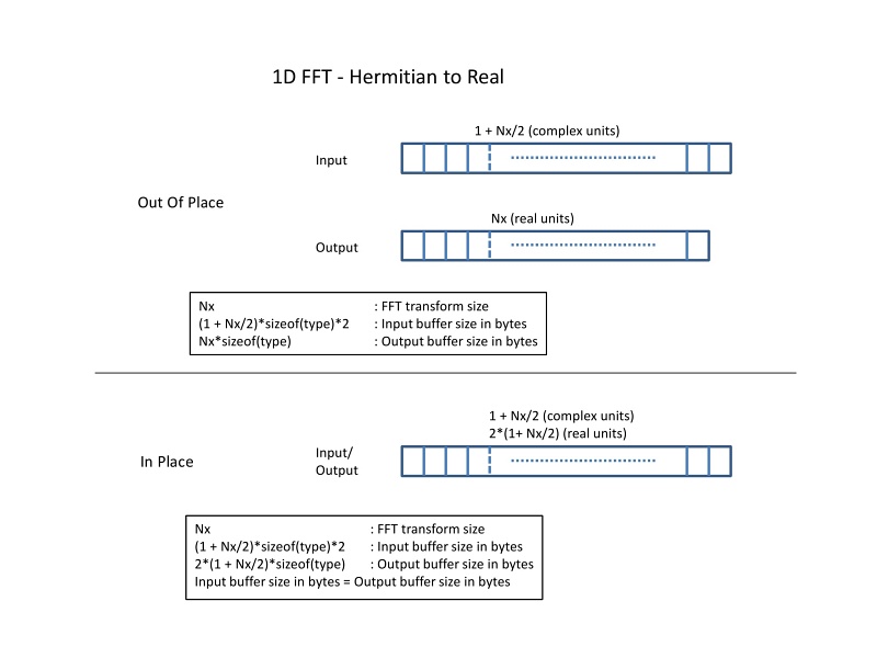
Fig. 9 1D FFT - Hermitian to real

Here is an example of an in-place transform with an even \(N\) and how strides and distances are set. Even though this example only deals with one buffer (in-place), the output strides/distance can take different values compared to the input strides/distance.

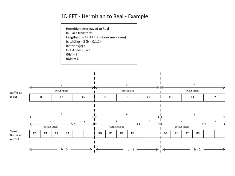
Fig. 10 1D FFT - Hermitian to real example

This schematic illustrates the in-place forward 2D FFT for real to Hermitian.

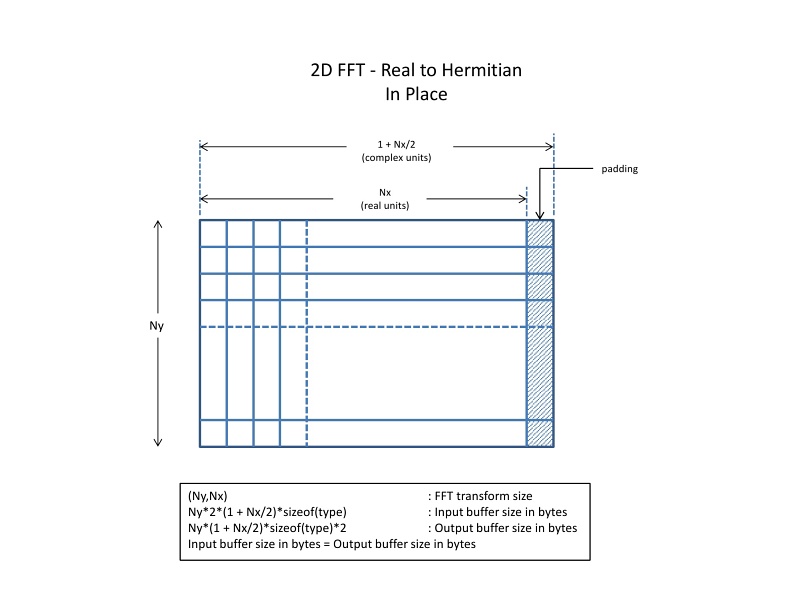
Fig. 11 2D FFT - Real to Hermitian in-place

Here is an example of an in-place 2D transform and how strides and distances are set. Even though this example only deals with one buffer (in-place), the output strides/distance can take different values compared to the input strides/distance.

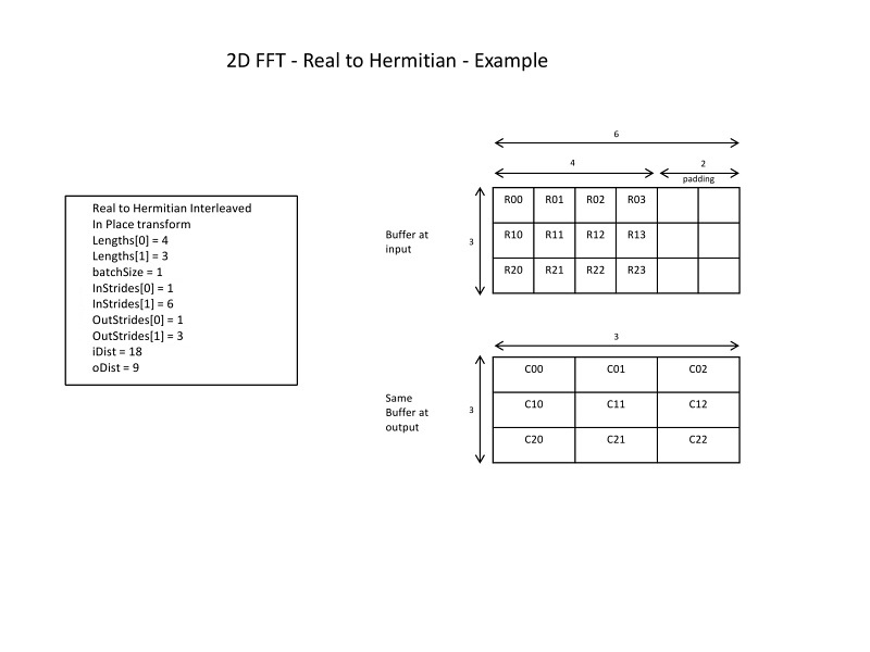
Fig. 12 2D FFT - Real to Hermitian example